Spatial hypotesis and autocorrelation Analysis
geospatial
map
hypotesis

Introduction
This project focuses on the one of critical part of exploratory spatial data analysis (ESDA), which is testing for spatial structure present within data.
Testing for spatial structure is important because if it is present in data, then we’ll want to leverage that spatial structure to enhance our downstream analysis. This can be done by using specialized algorithms during a model-building process that can understand patterns from both data and geographic space.
Theory
Spatial structure in simplest terms is the presence of a pattern within data across geographic space. Data that has no spatial structure is said to have been generated by an independent random process (IRP). This IRP result is data that exhibits complete spatial randomness (CSR).
Hypothesis testing is defined as a statistical test used to determine whether data supports a particular theory or hypothesis. A hypothesis test is broken out into a null hypothesis represented by H0 and an alternative hypothesis represented by Ha. with H0 The data is distributed randomly across space.
Spatial autocorrelation
Spatial autocorrelation measures the variation of a variable by taking an observation and seeing how similar or different it is compared to other observations within its neighborhood.
The notion of spatial autocorrelation relates to the existence of a
functional relationship between what happens at one point in space and what happens elsewhere.
Spatial autocorrelation thus has to do with the degree to which the similarity in values between observations in a dataset is related to the similarity in locations of such observations. Similar values are located near each other, while different values tend to be scattered and further away.
This is a fairly common case in many social contexts and, in fact, several human phenomena display clearly positive spatial autocorrelation (when observations within a neighborhood have similar values, either high-high values or low-low values). Conversely, negative spatial autocorrelation reflects a situation where similar values tend to be located away from each other.
Global spatial autocorrelation measures the trend in an overall dataset and helps we understand the degree of spatial clustering present. It considers the overall trend that the location of values follows. The study of global spatial autocorrelation makes possible statements about the degree of clustering in the dataset.
Do values generally follow a particular pattern in their geographical distribution? Are similar values closer to other similar values than we would expect from pure chance?
Local spatial autocorrelation, measures the localized variation in the dataset and helps we detect the presence of hot spots or cold spots. Hot spots are localized area clusters with statistically significant high values, and cold spots are localized area clusters with statistically significant lower values. Local autocorrelation focuses on deviations from the global trend at much more focused levels than the entire map.
Moran’s I statistic measures spatial autocorrelation of data based on feature values and feature locations.
Spatial weights and spatial lags
Spatial weights are used to determine the neighborhood for a given observation and are stored in a spatial weights matrix. There are three main spatial weights matrices:
- rook contiguity matrix: is created by taking the four nearest neighbors in a north, south, east, and west direction.
- queen contiguity matrix: is created by taking the eight nearest neighbors from every observation, in a similar fashion to how a queen moves about a chessboard.
- KNN matrix: is calculated for a given observation based on a set number of nearest neighbors, denoted as k. The number of nearest neighbors to use depends on (and will require a degree of exploration and domain knowledge of) the field or industry that the problem is based upon.
Spatial lag: is a variable that averages the values of the nearest neighbors, as defined by the spatial weights matrix chosen.
Row standardization: occurs by dividing the weight for a feature by the sum of all neighbor weights for that same feature. It is generally recommended that this process be applied any time there is potential bias due to the sampling construct or the aggregation process
LISAs are spatial statistics that are derived from global spatial statistics and calculate local cluster patterns, also known as spatial outliers. These spatial outliers are unlikely to appear if the assumption of spatial randomness was true.
Spatial autocorrelation for all parameters
Dataset
We’ll use a dataset contains an extract of a set of variables from the 2017 American Community Survey (ACS) Census Tracts for the San Diego (CA) metropolitan area.
db = gpd.read_file(r"..\map\sandiego_tracts.gpkg")
To make things easier later on, let us collect the variables we will use to characterize census tracts. These variables capture different aspects of the socioeconomic reality of each area and, taken together, provide a comprehensive characterization of San Diego as a whole.
cluster_variables = [
    "median_house_value",  # Median house value
    "pct_white",  # % tract population that is white
    "pct_rented",  # % households that are rented
    "pct_hh_female",  # % female-led households
    "pct_bachelor",  # % tract population with a Bachelors degree
    "median_no_rooms",  # Median n. of rooms in the tract's households
    "income_gini",  # Gini index measuring tract wealth inequality
    "median_age",  # Median age of tract population
    "tt_work",  # Travel time to work
]
The Code
By calling maps.spatial_autocorrelation_multi, we can measure Moran’s I value and P-value to determine spatial autocorrelation of data based on feature values and feature locations.
result = maps.spatial_autocorrelation_multi(main_data,col_list)
This function requires the following parameters:
- main_data (
string): Data location and value - col_list (
string): Targated column in main_data
The result
Moran’s I for each variable
| Variable | Moran’s I | P-value |
|---|---|---|
| median_house_value | 0.646618 | 0.001 |
| pct_white | 0.602079 | 0.001 |
| pct_rented | 0.451372 | 0.001 |
| pct_hh_female | 0.282239 | 0.001 |
| pct_bachelor | 0.433082 | 0.001 |
| median_no_rooms | 0.538996 | 0.001 |
| income_gini | 0.295064 | 0.001 |
| median_age | 0.38144 | 0.001 |
| tt_work | 0.102748 | 0.001 |
Each of the variables displays significant positive spatial autocorrelation, suggesting clear spatial structure in the socioeconomic geography of San Diego. This means it is likely the clusters we find will have a non-random spatial distribution.
Spatial autocorrelation for spesific variable
Dataset
For this project, we used 2 datasets:
- contains results for the Brexit vote at the local authority district, and administrative boundaries.
- the shapes of the geographical units, which downloaded from the Office of National Statistics through data.gov.uk
ref = pd.read_csv(r'..\map\bexit\EU-referendum-result-data.csv',index_col="Area_Code")

lads = gpd.read_file(r'E:\gitlab\dataset\map\bexit\local_authority_districts.geojson').set_index("lad16cd")
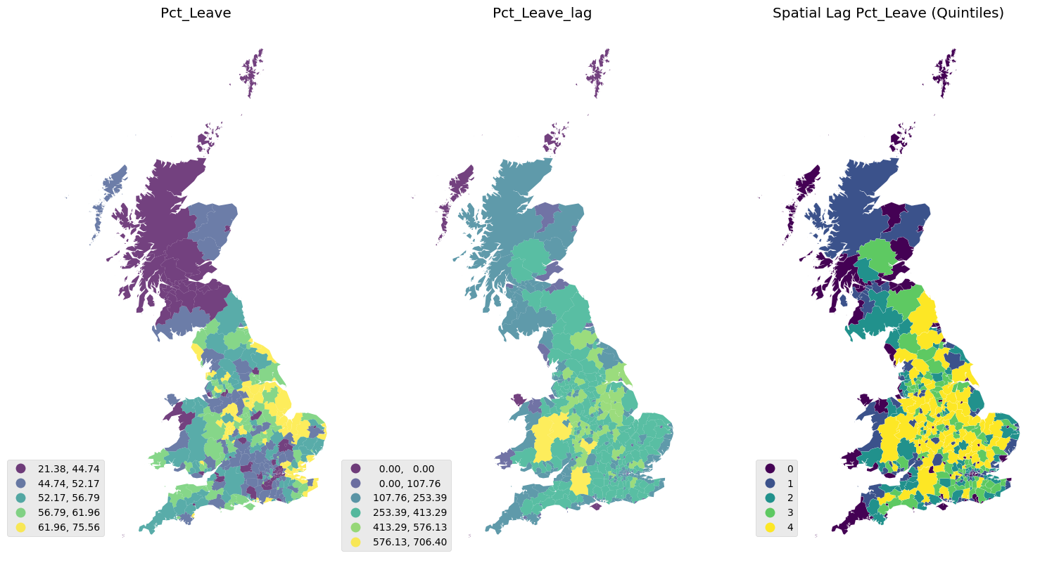
Although there are several variables that could be considered, we will focus on Pct_Leave, which measures the proportion of votes for the Leave alternative. For convenience, let us merge the vote results with the spatial data and project the output into the Spherical Mercator coordinate reference system (CRS).
db = (gpd.GeoDataFrame(lads.join(ref[["Pct_Leave"]]), crs=lads.crs)
    .to_crs(epsg=3857)[["objectid", "lad16nm", "Pct_Leave", "geometry"]]
    .dropna())
The Code
By calling maps.spatial_autocorrelation, we can measure Moran’s I value and P-value to determine spatial autocorrelation of data based on feature values and feature locations.
result = maps.spatial_autocorrelation(main_data, col_value='',
                            types='global',plot_spatial_lag=False,
                            getis_ord=False,num_quantiles=5)

res = maps.spatial_autocorrelation(db,col_value='Pct_Leave',
                             types='',plot_spatial_lag=True)

df, res = maps.spatial_autocorrelation(db,col_value='Pct_Leave',
                             types='global',plot_spatial_lag=False)

res = maps.spatial_autocorrelation(db,col_value='Pct_Leave',
                             types='local', plot_spatial_lag=False,
                             getis_ord=True)
This function requires the following parameters:
- main_data (
string): Data location and value - col_value (
string): Targated column in main_data - types (
string): Type of measurement (global, local) - plot_spatial_lag (
Boolean): Generate result plot - getis_ord (
Boolean): Measure getis order - num_quantiles (
Int): number quantiles
The result
Moran’s I for each variable
| lad16cd | objectid | lad16nm | Pct_Leave | geometry | Pct_Leave_lag | Pct_Leave_std | Pct_Leave_lag_std |
|---|---|---|---|---|---|---|---|
| E06000001 | 1 | Hartlepool | 69.57 | MULTIPOLYGON (((-141402.2145840305 7309092.065068442, -153719.06055720485 7293060.179709789, | 59.64 | 16.4292 | 7.59916 |
| E06000002 | 2 | Middlesbrough | 65.48 | MULTIPOLYGON (((-136924.09919632497 7281563.141098457, -142664.6188442458 7277835.885362477, | 60.5267 | 12.3392 | 8.48583 |
| E06000003 | 3 | Redcar and Cleveland | 66.19 | MULTIPOLYGON (((-126588.38167191816 7293641.927807655, -126076.00087943401 7286209.385436979, | 60.3767 | 13.0492 | 8.33583 |
| E06000004 | 4 | Stockton-on-Tees | 61.73 | MULTIPOLYGON (((-146690.6335327008 7293316.1435412755, -153719.06055720485 7293060.179709789, | 60.488 | 8.58924 | 8.44716 |
| E06000010 | 10 | Kingston upon Hull, City of | 67.62 | MULTIPOLYGON (((-35191.00877187259 7134866.243975437, -39368.88292597354 7133972.734487184, | 60.4 | 14.4792 | 8.35916 |
Global spatial autocorrelation
| types | global_value | p_sim | details | |
|---|---|---|---|---|
| 0 | moran_I | 0.724841 | 0.001 | positive spatial autocorrelation |
| 1 | geary_C | 0.32682 | 0.001 | positive spatial autocorrelation |
| 2 | getis_ord_G | 0.43403 | 0.001 | positive spatial autocorrelation |
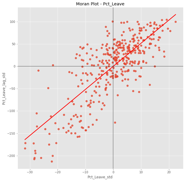
The plot displays a positive relationship between both variables. This is indicates the presence of positive spatial autocorrelation: similar values tend to be located close to each other. This means that the overall trend is for high values to be close to other high values, and for low values to be surrounded by other low values. This, however, does not mean that this is the only case in the dataset: there can of course be particular situations where high values are surrounded by low ones, and vice versa. But it means that, if we had to summarize the main pattern of the data in terms of how clustered similar values are, the best way would be to say they are positively correlated and, hence, clustered over space. In the context of the example, this can be interpreted along the lines of: local authorities where people voted in high proportion to leave the EU tend to be located nearby other regions that also registered high proportions of Leave vote. In other words, we can say the percentage of Leave votes is spatially autocorrelated in a positive way.
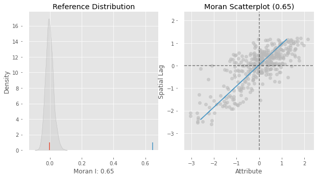
On the left panel we can see in grey the empirical distribution generated from simulating 999 random maps with the values of the Pct_Leave variable and then calculating Moran’s I for each of those maps. The blue rug signals the mean. In contrary, the red rug shows Moran’s I calculated for the variable using the geography observed in the dataset. It is clear the value under the observed pattern is significantly higher than under randomness. This insight is confirmed on the right panel, which shows an equivalent plot to the Moran Scatterplot we created above.
| lad16cd | objectid | lad16nm | Pct_Leave | geometry | Pct_Leave_lag | Pct_Leave_std | Pct_Leave_lag_std | moran_quadrant_outline | moran_p-sim | moran_sig | moran_labels | getis_ord_values | getis_ord_labels |
|---|---|---|---|---|---|---|---|---|---|---|---|---|---|
| E06000001 | 1 | Hartlepool | 69.57 | MULTIPOLYGON (((-141402.2145840305 7309092.065068442, -153719.06055720485 7293060.179709789, | 64.4667 | 16.4292 | 11.5224 | 1 | 0.182 | 0 | Non-Significant | 0 | LL (cold spots) |
| E06000002 | 2 | Middlesbrough | 65.48 | MULTIPOLYGON (((-136924.09919632497 7281563.141098457, -142664.6188442458 7277835.885362477, | 65.83 | 12.3392 | 12.8857 | 1 | 0.094 | 0 | Non-Significant | 0 | LL (cold spots) |
| E06000003 | 3 | Redcar and Cleveland | 66.19 | MULTIPOLYGON (((-126588.38167191816 7293641.927807655, -126076.00087943401 7286209.385436979, | 65.5933 | 13.0492 | 12.649 | 1 | 0.097 | 0 | Non-Significant | 0 | LL (cold spots) |
| E06000004 | 4 | Stockton-on-Tees | 61.73 | MULTIPOLYGON (((-146690.6335327008 7293316.1435412755, -153719.06055720485 7293060.179709789, | 63.7433 | 8.58924 | 10.799 | 1 | 0.058 | 0 | Non-Significant | 0.708221 | HH (hot spots) |
| E06000010 | 10 | Kingston upon Hull, City of | 67.62 | MULTIPOLYGON (((-35191.00877187259 7134866.243975437, -39368.88292597354 7133972.734487184, | 65.5233 | 14.4792 | 12.579 | 1 | 0.227 | 0 | Non-Significant | 0 | LL (cold spots) |
Local spatial autocorrelation
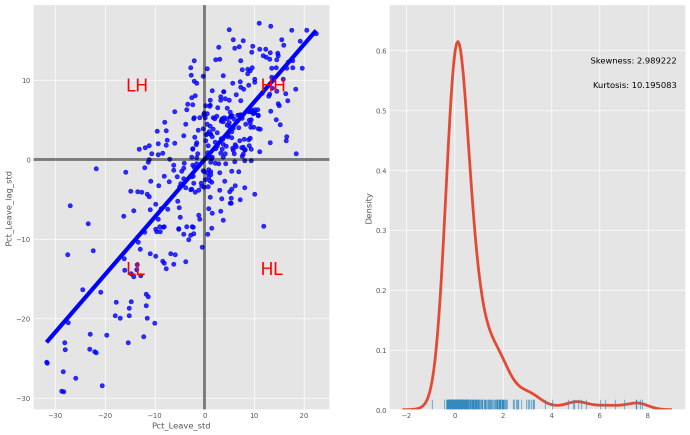
The figure reveals a rather skewed distribution of local Moran’s I statistics. This outcome is due to the dominance of positive forms of spatial association, implying most of the local statistic values will be positive. Here it is important to keep in mind that the high positive values arise from value similarity in space, and this can be due to either high values being next to high values or low values next to low values. The local I values alone cannot distinguish these two cases.
The values in the left tail of the density represent locations displaying negative spatial association. There are also two forms, a high value surrounded by low values, or a low value surrounded by high-valued neighboring observations. And, again, the I statistic cannot distinguish between the two cases.
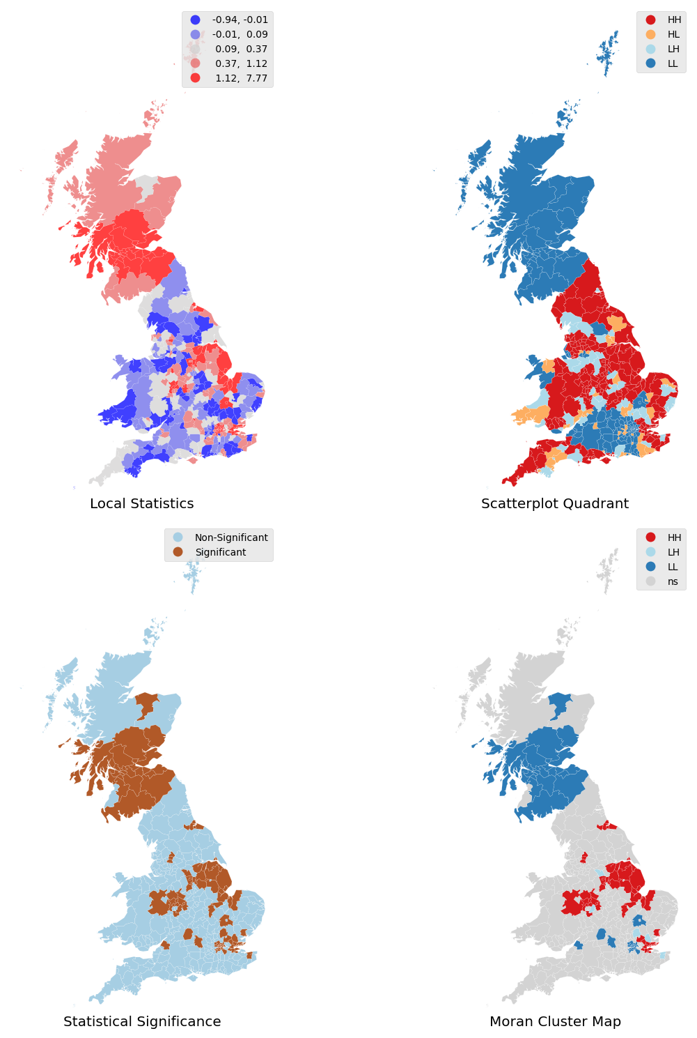
The red and blue locations in the top-right map in Figure 5 display the largest magnitude (positive and negative values) for the local statistics I. Yet, remember this signifies positive spatial autocorrelation, which can be of high or low values. This map thus cannot distinguish between areas with low support for the Brexit vote and those highly in favour.
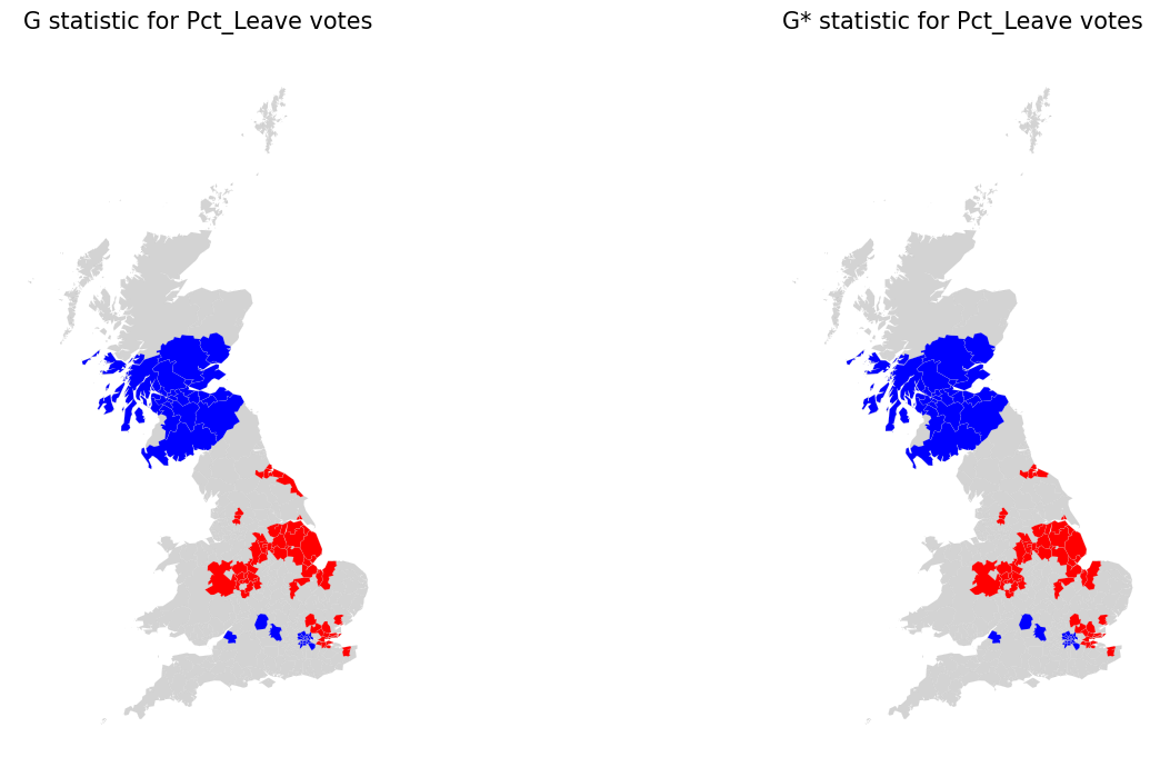
In this case, the results are virtually the same for Gi and Gi*. Also, at first glance, these maps appear to be visually similar to the final LISA map from above.
Table result
| moran_labels | count |
|---|---|
| Non-Significant | 274 |
| LL (cold spots) | 52 |
| HH (hot spots) | 49 |
| LH (doughnuts) | 5 |
| lad16cd | objectid | lad16nm | Pct_Leave | geometry | Pct_Leave_lag | Pct_Leave_std | Pct_Leave_lag_std | moran_quadrant_outline | moran_p-sim | moran_sig | moran_labels | getis_ord_values | getis_ord_labels |
|---|---|---|---|---|---|---|---|---|---|---|---|---|---|
| E06000001 | 1 | Hartlepool | 69.57 | MULTIPOLYGON (((-141402.2145840305 7309092.065068442, -153719.06055720485 7293060.179709789, | 64.4667 | 16.4292 | 11.5224 | 1 | 0.016 | 1 | HH (hot spots) | 1.09517 | HH (hot spots) |
| E06000002 | 2 | Middlesbrough | 65.48 | MULTIPOLYGON (((-136924.09919632497 7281563.141098457, -142664.6188442458 7277835.885362477, | 65.83 | 12.3392 | 12.8857 | 1 | 0.006 | 1 | HH (hot spots) | 1.22369 | HH (hot spots) |
| E06000003 | 3 | Redcar and Cleveland | 66.19 | MULTIPOLYGON (((-126588.38167191816 7293641.927807655, -126076.00087943401 7286209.385436979, | 65.5933 | 13.0492 | 12.649 | 1 | 0.007 | 1 | HH (hot spots) | 1.20137 | HH (hot spots) |
| E06000004 | 4 | Stockton-on-Tees | 61.73 | MULTIPOLYGON (((-146690.6335327008 7293316.1435412755, -153719.06055720485 7293060.179709789, | 63.7433 | 8.58924 | 10.799 | 1 | 0.026 | 1 | HH (hot spots) | 1.02105 | HH (hot spots) |
| E06000010 | 10 | Kingston upon Hull, City of | 67.62 | MULTIPOLYGON (((-35191.00877187259 7134866.243975437, -39368.88292597354 7133972.734487184, | 65.5233 | 14.4792 | 12.579 | 1 | 0.007 | 1 | HH (hot spots) | 1.19558 | HH (hot spots) |